Analysis of the statistical distribution of the population in terms of average per capita money income. Distribution of the population on average per capita income distribution of the population by the magnitude of the average
| Environmental cash income | Total income. | |||||
| , rub. | in% to the outcome | |||||
| All population,% | ||||||
| Including with the average foreign monetary income per month, rub. | ||||||
| up to 400. | 15,1 | 15,1 | 4,9 | 4,9 | ||
| 400,1-600 | 19,0 | 34.1 | 10.2 | 15,1, | ||
| 600.1-800 | 17,2 | 51,3 | 12,9 | 28,0 | ||
| 800,1-1000 | 13,3 | 64,6 | 12,9 | 40,9 | ||
| 1000,1-1200 | 9.8 | 74,4 | 11,6 | 52.5 | ||
| 1200.1-1600 | 12,0 | 86,4 | 18.0 | 70.5 | ||
| 1600,1-2000 | 6.1 | 92,5 | 11.8 | 82.3 | ||
| Over 2000. | 7,5 | 17,7 | ||||
| Note. . A source. Russian statistical yearbook. 1999: Statistical compilation. -M.: Goskomstat Russia, 1999. - P. 155. |

where is the I-th decile;
Decile's room (nine decays are calculated); - Lower border interval , Containing
i-th decile (defined by the accumulated general);
The magnitude of the income interval;
- the coefficient corresponding to the decill number: for for, with;
The amount of aggregate (the total population);
Accumulated frequency in the interval preceding the interval containing the I-th decile;
The frequency of the interval containing the I-th decile.
Based on data Table. 5.7 The first decile is located in the first interval.
![]()
First decil 332,55 rubles. characterizes the maximum income of 10% of the least wealthy population. Ninth Decil, located in the penultimate interval,
characterizes the minimum income of 10% of the most wealthy population.
Coefficient of income differentiation (decyl) \u003d
![]()
showing that 5.5 times the minimum income of 10% of the most wealthy population exceeds the maximum income of 10% of the least wealthy population,
Fund coefficients (the relationship between average income values \u200b\u200binside compared extreme decile groups of the population or their shares in the total volume of income) is calculated by non-grouped data.
The disadvantage of the dezyl coefficient of differentiation and the factor of funds is the partial use of information distribution information on income only within the framework of extreme decile groups. To study the differentiation of income throughout the distribution, there are regrouping of the population through quintile groups, uniting by 20% of the population. For each selected group, the share in total income is calculated.
The example of the calculation of quintiles (K), dividing a combination of five equal parts (quintile four):
characterizes the maximum income of 20% of the poor

characterize the minimum income of 20% of the most wealthy population. The values \u200b\u200bof quintile show the boundaries of the intervals, in each of which focused on 20% of the population. In technical frequencies, the accumulated consumption of cumulative income is calculated:
such a share of total income has 20% of the least poor;
accumulated frequency - such a share of the total monetary beforethe course has 40% of low-income population;

The calculations of quintile and the accumulated frequency of money revenue will be issued in Table. 5.8.
Based on the data obtained, the income differentiation is reflected in the most clearly: 20% of the poor are 7.8% of the total monetary income of society, and 20% of the rich population - 39.1% of the total monetary income.
Differentiation indicators generalizing all distribution of population in income include the coefficients of the concentration of Lorentz and Gini's income. They refer to the rating system known as the Pareto-Lorentz-Gini methodology, widely used in foreign social statistics. The Italian economist and sociologist V. Pareto (1848-1923) summarized the data of some countries and found that there is an inverse relationship between the level of income and the number of their recipients, called Pareto law. American statistics and economist O, Lorenz (1876-1959) developed this law, offering its graphic image in the form of a curve, called the "Lorentz curve" (Fig. 5.2).
Table5.8.
Distribution of money income by 20% to population groups
| Quintle group of the population | To the result | Accumulated money income | Share of income to the outcome | ||
| Money profit just | 1.0 | 1,000 | 0,200 | 0,4492 | |
| Including 20% \u200b\u200bgroups of the population: | |||||
| First group (with the least income) | 0.2 | 0,078 | 0,0156 | 0.01 | |
| Second group | 0,2 | 0.195 | 0,117 | 0.0234 | 0.0390 |
| Third Group | 0,2 | 0,364 | 0,169 | 0.0338 | 0,0728 |
| Fourth group | 0.2 | 0.609 | 0,245 | 0,0490 | 0,1218 |
| Fifth group | 0,2 | 1,000 | 0,391 | 0,0782 | 0,2000 |
Lorentz curve is a concentration curve by groups. Lorentz's reinforcement in the event of a uniform distribution of income pairwise shareholders and income should coincide and are located on the square diagonal, which means the complete absence of income concentration. Songs of direct connecting points corresponding to the accumulated generals and increasing income percentages form a broken concentration line (Lorentz curve). The more this line differs from the diagonal (the more its concave), the greater the unevenness of the income distribution, respectively, above its concentration.
Obviously, in specific cases, it is impossible to expect neither absolutely equality or absolute inequality in the distribution of income among the population. Absolute inequality is the hypothetical case, when the entire population, with the exception of one person (one family), has no income, and this one (one family) receives all income.

Fig. 5.2. Curve Lorentz
An example of building a Lorentz schedule:
the accumulated frequency of the population (abscissa axis) is 0.20,40,60,80,100;
the accumulated frequency of income (ordinate axis): with absolute equality - 0, 20, 40, 60,80, 100;
with absolute inequality - on the axis, the ordinates would be 0.0.0.0.0, 100; actually turned out to be 8; twenty; 36; 61; 100.
Lorentz coefficient as a relative characteristic and equality in income distribution
where is the share of revenues focused on the Ith social group;
The share of the population belonging to the I-th social group in the total population;
Number of social groups.
Extreme values \u200b\u200bof the Lorentz coefficient: in case of complete equality in the distribution of income; - with full inequality.
According to Table. 5.8 Lorentz coefficient
i.e. income distribution close to uniform.
On relative inequality in the income distribution may indicate the proportion of the area of \u200b\u200bdeviation from the uniform distribution (absolute pectorism, i.e. the area of \u200b\u200bthe segment formed by the Lorentz curve and the square diagonal, in half the square of this square).
![]()
where is the cumulative share of income.
The G coefficient varies in the range from 0 to 1. The closer the value to 1, the higher the level of inequality (concentration) in the distribution of cumulative income; The closer it to 0, the higher the level of equality. Calculate the coefficient can be calculated according to Table. 5.8.
Gini coefficient in Russia amounted to: in 1992 - 0.289; In 1993 - 0.398; In 1994 - 0.409; In 1995 - 0.381; In 1998 - 0.379. The overall increase in the coefficient for 1992 - 1998. He indicates an increase in inequality in the distribution of cumulative income in society.
Another meter of differentiation of income, in a broader sense - and social inequality, was proposed in 1970 by the British economist A. Atkinson and in modern economic literature, the name of the Atkinson index was based on the Atkinson index, imposing an equivalent income, i.e. the smallen cumulative The average per capita income, which, with a uniform distribution of income, would lead to the same magnitude of social welfare as with the existing income inequality. Public welfare, in turn, is defined as the amount of individual utility of members of society:
![]()
where - the individual functions of utility that in the Atkinsonic index only from the income of the individual and are relations:
![]()
(here - income i-GO Individual: - Constant).
Accounting when building an Atkinson index of such categories as public welfare and utility functions, allows you to interpret this indicator as a measure of social inequality. However, the fact that individual utility functions depend only on income, leads to the fact that in empirical calculations, social inequality is reduced essentially to the inequality of income of the population.
In accordance with the definition of equivalent income, we have:
Hence (taking into account the type of individual utility function)
![]()
![]()
Atkinson's index is defined

where is the average income.
The term, which in this index is subtracted from 1, characterizes the share of the equivalent level of income in the average per capita income. In other words, this term shows what proportion of aggregate income is the increasing distribution of which among all members of society would achieve existing well-being in society. In the last formula, this term is a power-weighted average of the income of each group in average income. Sounds of the distribution of the population in terms of income usually have a right-sided asymmetry, the greatest share in a number of distribution will have a share, as a result of which the average share will also be less than 1. With full equality of income, all relations would be equal to 1, and the Atkinson index would be 0. So, the Atkinson index is relative (in the shares of the cumulative wealth) the expression of the price that society pays for the existing level of social inequality.
The main disadvantage of the Atkinson index is that it is not difficult to set the value of the parameter, and it is impossible to find a solution to this problem. With this parameter, the Atkinson index allows us to take into account the importance for the inequality society in the distribution of public wealth. If society is absolutely indifferent to existing inequality, then e. \u003d 0. In this case, the Atkinson index value is also 0, since the average share of the income of each group in the average per capita income is calculated using the formula of the average arithmetic weighted and takes the value 1. If, on the contrary, society worries the only problem - social inequality, the parameter is rushed to Infinity. In accordance with the rule of majority of medium with increasing E (with other things being equal), the average share of the income of each group in the average per capita income will decrease in aspiration e. To infinity, strive for zero. Thus, in the hypothetical situation, when society worries exclusively on the problems of redistribution of income, the situation of low-income groups and the decrease in inequality, the Atkinson index will be close to 1. Any other value in the interval from 0 to 1 defines the importance of the society of redistribution processes in favor of the least secured Layers of the population. In tab. 5.9 The values \u200b\u200bof the Atkinson index calculated according to the data distribution of the population on average per capita income in 1995 are given for various values \u200b\u200be. For example, at e \u003d 1.5, the benefit derived from the redistribution of income in favor of its uniform distribution in 1995, It would be equivalent to an increase in total income by 0.281, or by 28.1%.
To calculate the analysis of the statistical distribution of the population by the magnitude of the average per capita cash income, it is necessary to close the first and last intervals and make a subsidiary table, where:
- - the number of man (in percent);
- - middle interval;
- - accumulated frequencies.
Table 6 - distribution of population in terms of average percentage income (in percent)
Figure 2.7 - distribution of the population in the Russian Federation by the magnitude of the average per capita cash income in 2013
As can be seen from the data submitted, the largest population of 31.3% has an average per month per month over 25 thousand rubles. Next follows a group of income from 15 thousand rubles. up to 25 thousand rubles. (28.8%) and closes the Troika district population group with an income of 10 thousand rubles. up to 15 thousand rubles. (20.0%).
Table 7 - Auxiliary Table

Figure 2.8 - Cumulating population distribution by the magnitude of the average per capita income
- 1. Determine the indicators of the distribution center:
- 1.1) Average arithmetic:
Based on these subsidiary table, the Fashion is 25.74 thousand rubles. The modal interval is selected for the calculation (25,000 rubles. up to 35,000 rubles), since it has the greatest frequency (31.3%). Thus, the most common average of the average per capita income in the variational series is 25,740 rubles.
1.3) Mediana
The median interval is selected for the calculation, in which the amount of accumulated frequencies is more than 50% (from 15,000 rubles. Up to 25,000 rubles). Consequently, half of the inhabitants of the Russian Federation have a monthly average income less than $ 2143.1 rubles, and half more than this amount.
- 2. Determine the indicators of the variation:
- 2.1) Variation variation
- 2.2) Medium linear deviation
weighted:

2.3) secondary quadratic deviation
weighted:

2.4) Dispersion
weighted:

2.5) Camefficient of Variation
- - Variation medium, aggregate relatively homogeneous
- 3. Determine the distribution form indicators:
- 3.1) asymmetry coefficient
asymmetry significant, right-sided
1) Determine the Decile Differentiation Coefficient
To determine the deceyl amount of differentiation of income of the Russian Federation, it is necessary to calculate the upper and lower decil.
4.1) Lower Decile

Approximately 10% of the population of the Russian Federation in 2013 had wages less than 7353.8 rubles.
4.2) Upper Decile
income population costs
Approximately 10% of the Russian Federation in 2013 had wages more than 31805.1 rubles.
4.3) Decile Differentiation Coefficient
In 2013, the minimum monthly average income of 10% of the most secured population exceeds the maximum income of 10% of the least secured population by 4.3 times.
The distribution of the population in terms of average per capita cash income
Revenue policy. Curve Lorentz. Zhini Index
This requires the transformation of the problem of combating poverty into one of the priority objectives of the state at the present stage of socio-economic development.
The main task of a socially oriented economy, the creation of which is proclaimed in our country, it is the achievement of human well-being.
Welfare- ϶ᴛᴏ Security of the population necessary for the life of material and spiritual benefits.
Revenues (Income) - cash resources entering a subject as a result of the distribution of ND, which are used by the subject for the needs.To estimate the level and dynamics of the received income use indicators nominal and real income.
Nominal income - this isquantity Money, obtained in a certain period of a separate person (ZP, capital income, transfer payments).
Real income - this is the number of goods and services, ĸᴏᴛᴏᴩᴏᴇ can be bought at current prices on the disposable income in a certain period of time.
Income population - A combination of revenues in the monetary and natural form received by a person, family, a household from various sources during a certain period of time (month, year) spent on consumption, accumulation, payment of taxes, the implementation of other fees and payments.
Transfer plates - various gratuitous payments to the population from public funds, in particular pensions, scholarships, various social benefits.
The composition of the monetary income of the population (in (%)
| Monetary income - all | |||||||||||||
| including: | |||||||||||||
| Salary | 83,3 | 79,8 | 76,4 | 62,8 | 62,8 | 64,6 | 65,8 | 63,9 | 65,0 | 63,6 | 64,9 | 70,4 | |
| Entrepreneurial income | 2,5 | 2,2 | 3,7 | 16,4 | 15,4 | 12,6 | 11,9 | 12,0 | 11,7 | 11,4 | 11,1 | 10,0 | |
| Social payments | 12,6 | 15,1 | 14,7 | 13,1 | 13,8 | 15,2 | 15,2 | 14,1 | 12,8 | 12,7 | 12,0 | 10,9 | |
| Revenues from property | 0,6 | 1,3 | 2,5 | 6,5 | 6,8 | 5,7 | 5,2 | 7,8 | 8,3 | 10,3 | 10,0 | 6,7 | |
| Other incomes | 1,0 | 1,6 | 2,7 | 1,2 | 1,2 | 1,9 | 1,9 | 2,2 | 2,2 | 2,0 | 2,0 | 1,9 | |
Revenue policy - The policy of controlling inflationary processes by restrictions on wage growth and other types of income.
State policy income It consists in redistributing them through the state budget by differentiated taxation of various groups of revenue receipts and social benefits.
The state policy of income is an integral part of social policy and is aimed at solving two main tasks:
1) the provision of direct assistance to the most vulnerable layers of the population through the social security system;
2) neutralization of inflationary depreciation of income and population savings.
| All population | ||||
| including with average money mining per month, rub.: | ||||
| up to 2000.0. | 12,3 | 7,1 | 4,3 | 2,6 |
| 2000,1 - 4000,0 | 28,1 | 21,9 | 16,2 | 11,9 |
| 4000,1 - 6000,0 | 21,1 | 20,3 | 17,7 | 14,9 |
| 6000,1 - 8000,0 | 13,4 | 14,8 | 14,7 | 13,6 |
| 8000,1 - 10000,0 | 8,4 | 10,3 | 11,2 | 11,3 |
| 10000,1 - 15000,0 | 10,0 | 13,9 | 17,1 | 19,1 |
| 15000,1 - 25000,0 | 5,2 | 8,6 | 12,7 | 16,5 |
| Over 25000.0. | 1,5 | 3,1 | 6,1 | 10,1 |
To measure the degree of inequality in society in practice, a number of methods are used, and one of the most famous is considered curve Lorentz graphically representing information about the distribution of income of various groups of the population.
Curve Lorentz - the curve showing what part of the country's total cash income receives every share of low-income and high-yield families, that is, reflects in%-one distribution of income between families with different sufficiency.
Max Otto Lorentz(1876-1959) - American economist.
| Revenues (%) 100 ● 80 Absolute Equality is actual 60 distribution revenues 40 Absolute 20 inequality B 0 ● ● Pass (%) 20 40 60 80 100 Fig. Curve Lorentz. |
Curve Lorentzshows the uneven distribution of the cumulative income of society between various groups of the population.
Lorentz curve before tax deductions
20 and accounting transfer payments
0 Pass (%)
Quantitative indicator of the level of uneven income distribution is gini coefficient, or concentration coefficient.
Korrado Gini. (1884-1965) - Italian statistics and demographer.
Gini coefficient (income concentration index) - characterizes the degree of deviation of the line of actual distribution of the total volume of the income of the population from the line of their uniform distribution.
The magnitude of the coefficient of Gini May vary from 0 before 1, At the same time, the higher the value of the indicator, the more unevenly distributed income in society.
It is defined as the ratio of the area between the Lorentz curve and the diagonal to the area of \u200b\u200bthe triangle of ATS, ᴛ.ᴇ. Sets the degree of deviation of the actual distribution of income from uniform.
| Gini coefficient (income concentration index) | 0,387 | 0,395 | 0,397 | 0,397 | 0,403 | 0,409 | 0,406 | 0,410 | 0,415 |
The advantages of the Gini coefficient:
‣‣‣ allows you to compare the distribution of the feature in aggregates with different numbers of units (eg: regions with different population of the population).
‣‣‣ complements data on GDP and average per capita income. It serves as a kind of correction of these indicator.
‣‣‣ can be used to compare the distribution of a sign (income) between different collapsions (for example: by different countries). There is no dependence on the scale of the economy of the compared countries.
‣‣‣ can be used to compare the distribution of a trait (income) in different groups of the population (eg: the Gini coefficient for the rural population and the Gini coefficient for the urban population).
‣‣‣ Allows you to track the dynamics of the uneven distribution of the sign (income) in the aggregate at different stages.
‣‣‣ Anonymity is one of the main advantages of the Gini coefficient. No, it is extremely important to know who has what income personally.
Disadvantages of the Gini coefficient:
‣‣‣ Quite often, the Gini coefficient is given without a description of the grouping of the aggregate, that is, there is often no information on what kind of quantili was given a combination. So, by a larger number of groups, the same totality (more quantile) was given, the higher the value of the Gini coefficient.
‣‣‣ The coefficient of Gini does not take into account the source of income, that is, for localization (country, region, etc.), the Gini coefficient must be quite low, but at the same time some part of the population provides its income due to the unbearable labor, and Another - at the expense of property. Thus, in Sweden, the value of the Gini coefficient is quite low, but at the same time only 5% of households own 77% of shares from the total number of shares, which are owned by the household. This ensures this 5% income that the rest of the population gets due to labor.
Efficiency e Fig. Reforming the Russian economy.
The distribution of the population in terms of average per capita cash income is the concept and types. Classification and features of the category "Distribution of the population in terms of average per capita cash income" 2017, 2018.
Modal income is the most common income among the population. This indicator is determined by the formula:
Where is the lower limit of the modal interval; - the magnitude of the interval; - frequency of the modal interval; - frequency preceding the modal interval; - frequency of the postmodal interval.
The median income is an income that characterizes that half of the population has an income below the median, and half of the population has an income above the median.
 (37)
(37)
Where is the lower boundary of the median interval; - the magnitude of the median interval; - the sum of all frequencies; - the frequency of the median interval; - accumulated frequency of the premedicated interval.
Fund coefficients are the ratio between average incomes of 10% of the richest population and 10% of the poorest population of the country, i.e. The ratio of income in the tenth and first decyl groups.
The concentration coefficient of Gini's income characterizes the degree of inequality in the distribution of income of the country's population and is calculated by the formula:
Where - the proportion of the population that has income higher than its maximum level in the 1st group, i.e. increasing share of the population; - increasing share of income of the population.
The Gini coefficient varies in the range from 0 to 1. The closer to 1, the higher the stratification of the Company in income, i.e. Most of the income is concentrated in a small population group.
The distribution of the population in terms of average per capita cash income in the Chuvash Republic is presented in Table 47.
Table 47. - distribution of the population in terms of average
cash income (in percent)
| Indicators | Years | |||||||||
| All population | ||||||||||
| including with average foreign cash income, rubles per month | ||||||||||
| up to 1000.0. | 51,7 | 30,4 | 16,3 | 8,1 | 5,6 | 2,6 | 1,1 | 0,5 | 0,2 | 0,1 |
| 1000,1-1500,0 | 26,3 | 28,1 | 22,9 | 15,5 | 12,1 | 7,4 | 3,8 | 2,0 | 0,9 | 0,6 |
| 1500,1-2000,0 | 12,2 | 18,3 | 19,8 | 17,1 | 14,7 | 11,0 | 6,4 | 3,8 | 2,0 | 1,5 |
| 2000,1-3000,0 | 7,7 | 16,0 | 23,5 | 26,5 | 25,8 | 23,5 | 16,7 | 11,8 | 7,4 | 5,9 |
| 3000,1-4000,0 | 1,6 | 4,8 | 10,0 | 15,2 | 16,9 | 18,6 | 16,5 | 13,7 | 10,1 | 8,6 |
| 4000,1-5000,0 | 0,3 | 1,5 | 4,1 | 8,0 | 10,0 | 12,8 | 13,7 | 12,9 | 10,8 | 9,8 |
| 5000,1-7000,0 | 0,1 | 0,7 | 2,6 | 6,5 | 9,3 | 13,7 | 18,5 | 20,2 | 19,5 | 18,7 |
| 7000,1-12000,0 1) | 0,1 | 0,2 | 0,8 | 2,8 | 4,9 | 8,8 | 17,4 | 23,7 | 28,9 | 30,3 |
| Over 12000.0. | - | - | - | 0,3 | 0,7 | 1,6 | 5,9 | 11,4 | 20,2 | 24,5 |
1) 2000 - 2002. - Over 7000 rubles.
Based on the data presented above, we construct an auxiliary table 48 and calculate a number of indicators characterizing the differentiation of income of the population in 2000.
Table 48 - Auxiliary Table
| Fisher income per month, rub. | The proportion of the population to the result, | Middle interval | Increasing frequency of the population | Share of revenues to the result | Increasing interests of income, | |||
| up to 1000.0. | 0,517 | 0,517 | 258,500 | 0,240 | 0,240 | 0,282 | 0,187 | |
| 1000,1-1500,0 | 0,263 | 0,78 | 328,750 | 0,305 | 0,545 | 0,579 | 0,491 | |
| 1500,1-2000,0 | 0,122 | 0,902 | 213,500 | 0,198 | 0,743 | 0,831 | 0,727 | |
| 2000,1-3000,0 | 0,077 | 0,979 | 192,500 | 0,179 | 0,921 | 0,953 | 0,917 | |
| 3000,1-4000,0 | 0,016 | 0,995 | 56,000 | 0,052 | 0,973 | 0,981 | 0,971 | |
| 4000,1-5000,0 | 0,003 | 0,998 | 13,500 | 0,013 | 0,986 | 0,989 | 0,985 | |
| 5000,1-7000,0 | 0,001 | 0,999 | 6,000 | 0,006 | 0,991 | 0,999 | 0,991 | |
| 7000,1-12000,0 2) | 0,001 | 9,500 | 0,009 | 1,000 | 1,000 | 1,000 | ||
| Over 12000.0. | 0,000 | 0,000 | 1,000 | 0,000 | 0,000 | |||
| TOTAL | 1078,250 | 1,000 | 6,613 | 6,269 |
Decision.
1. Calculate the average per month per month:
![]()
2. MODAL INCOME:
3. Median income:
![]()
4. Middle income in decile groups.
Lower Decile (the lowest income):
![]()
Upper decil (highest income):
5. Fund coefficients:
![]()
Consequently, in 2000, the average incomes of 10% of the richest people had revenues exceeding 10.3 times the income of the poorest people.
6. Gini revenue ratio:
Order procedure the values \u200b\u200bof the subsistence minimum And his appointment is regulated by the Federal Law of October 24, 1997 No. 134-FZ "On the subsistence minimum in the Russian Federation". According to the law, the amount of the subsistence minimum is a cost assessment of the consumer basket, as well as mandatory payments and fees.
Consumer basket includes minimal sets of food, non-food and services needed to preserve human health and ensure its livelihoods.
The consumer basket is developed both in Russia as a whole and in the constituent entities of the Russian Federation for the three socio-demographic groups of the population: able-bodied population, retirees and children. In general, in Russia, it is established by federal law, and in the constituent entities of the Russian Federation - legislative acts of the constituent entities of the Russian Federation.
Consumer Basket Food Set includes: Bread products, Potatoes, Vegetables and Bakhchy, Fruits Fresh, Sugar and confectionery, Meat products, fish products, milk and milk products, Eggs, Vegetable oil, Margarine and other fats, Other products (salt , tea, spices).
When forming a minimum set of food, the norms of physiological needs for foodstatons for the working-age, pensioners and children, as well as the recommendations of the World Health Organization are used.
A set of non-food products included in the consumer basket includes customized goods (clothing, shoes, school-writing goods) and public-place goods (bed linen, consumer and economic goods, essentials, sanitation and medicine).