starting with and continuing with the mentioned k terminals.

A grammar is called an LL(k)-grammar if it is an LL(k)-grammar for some k.

Example 4.7. Consider grammar G = ((S, A, B), (0, 1, a, b), P, S), where P consists of rules

S -> A | B, A -> aAb | 0, B -> aBbb | one.

Here . G is not an LL(k)-grammar for any k. Intuitively, if we start by reading a long enough string of characters a , we don't know which of the rules S -> A and S -> B was applied first until we encounter 0 or 1 .

Turning to the precise definition of the LL (k)-grammar, we set and y = a k 1b 2k . Then the conclusions

correspond to conclusions (1) and (2) of the definition. The first k characters of strings x and y match. However, the conclusion is false. Since k is chosen arbitrarily here, G is not an LL grammar.

Consequences of the definition of LL(k)-grammar

Theorem 4.6. CS Grammar is an LL(k)-grammar if and only if for two different rules and from R intersection empty for all such , what .

Proof. Need. Assume that and satisfy the conditions of the theorem, and contains x . Then, by the definition of FIRST, for some y and z there are conclusions

(Note that here we have used the fact that N does not contain useless non-terminals, as is assumed for all the grammars under consideration.) If |x|< k ; то y = z = e . Так как , то G не LL (k)- грамматика .

Adequacy. Assume that G is not an LL(k)-grammar.

Then there are two conclusions

that the strings x and y match in the first k positions, but . Therefore, and are different rules from P and each of the sets and contains the string FIRST k (x) that matches the string FIRST k (y) .

Example 4.8. A grammar G consisting of two rules S -> aS | a , will not be an LL(1)-grammar, since

FIRST 1 (aS) = FIRST 1 (a) = a.

Intuitively, this can be explained as follows: when parsing a string that begins with the character a , we see only this first character, we do not know which of the rules S -> aS or S -> a should be applied to S . On the other hand, G is an LL(2)-grammar. Indeed, in the notation of the theorem just presented, if , then A = S and . Since only two specified rules are given for S, then and . Since FIRST2(aS) = aa and FIRST2(a) = a , then by the last theorem G is an LL (2)-grammar.

Removing left recursion

The main difficulty in using predictive analysis is finding a grammar for the input language that can be used to build an analysis table with uniquely defined inputs. Sometimes, with some simple transformations, a non-LL(1) grammar can be reduced to an equivalent LL(1) grammar. Among these transformations, left factorization and left recursion removal are the most efficient. Two remarks must be made here. Firstly, not every grammar becomes LL(1) after these transformations, and secondly, after such transformations, the resulting grammar may become less understandable.

Immediate left recursion, that is, recursion of the form , can be removed in the following way. First, we group the A-rules:

where none of the lines start with A . Then we replace this set of rules with

where A" is a new non-terminal. The same chains can be derived from non-terminal A as before, but now there is no left recursion. This procedure removes all immediate left recursions, but does not remove left recursion involving two or more steps. Given below algorithm 4.8 allows you to remove all left recursions from the grammar.

Algorithm 4.8. Removing left recursion.

entrance. COP-grammar G without e-rules (of the form A -> e ).

Exit. COP-grammar G" without left recursion, equivalent to G .

Method. Follow steps 1 and 2.

(1) Arrange the non-terminals of the grammar G in an arbitrary order.

(2) Perform the following procedure:

After the (i-1) th iteration of the outer loop at step 2 for any rule of the form , where k< i , выполняется s >k . As a result, at the next iteration (by i ), the inner loop (by j ) sequentially increases the lower bound by m in any rule until m >= i . Then, after removing the immediate left recursion for A i -rules, m becomes greater than i .

With a top-down recursive parsing procedure, the problem of an infinite loop can arise.

In a grammar for arithmetic operations, applying the second rule will cause the parsing procedure to loop. Such grammars are called left-recursive. A grammar is said to be left-recursive if it contains a non-terminal A for which there is a derivation A=>+Aa. In simple cases, left recursion is called by rules of the form

In this case, a new non-terminal is introduced and the original rules are replaced by the following ones.

(if there is a non-terminal A for which there is an output A→+Aa in 1 or more steps). Left recursion can be avoided by transforming the grammar.

For example, productions A→Aa

Can be replaced with the equivalent:

For such a case, there is an algorithm that excludes left recursion:

1) define some order on the set of non-terminals (А 1 , А 2 , …, А n)

2) we take each non-terminal if there is a production for it that takes into account the non-terminal to the left, and transform the grammar:

for i:=1 to n do

for j:=1 to i-1 do

if Ai → Ajγ then Ai→δ1γ

│ δkγ, where

Aj → δ1│ δ2│ …│ δk

3) exclude all cases of direct left recursion (rule 1)

That. algorithm helps to avoid looping.

Elimination of left recursion from the grammar of arithmetic expressions and the general form of the rule for excluding left recursion:

General view of the left recursion exclusion rule

Left factorization.

LL(1) grammars are needed in order to select the right production for parsing from top to bottom, so that looping does not occur.

Sometimes it is possible to convert the grammar to LL(1) form using the left factorization method.

For example: S → if B then S

│if B then S else S

These productions violate the condition of LL(1)-grammars. This grammar can be converted to the form LL(1).

S → if B then S Tail

V general view this transformation can be defined like this:

we introduce a new non-terminal B, for which

| β N Left factorization can be applied to B. This procedure is repeated as long as the choice of products remains uncertain (ie, until something can be changed in it).

Building the FIRST Set

The First set for a non-terminal defines the set of terminals that this non-terminal can start with.

1. If x is a terminal, then first(x)=(x). Since the first character of a sequence from one terminal can only be the terminal itself.

2. If the grammar contains the rule Хà e, then the set first(х) includes e. This means that X can start with an empty sequence, that is, it can not exist at all.

3. For all productions of the form XàY1 Y2 … Yk we do the following. We add to the set first(X) the set first(Yi) until first(Yi-1) contains e and first(Yi) does not contain e. In this case, i changes from 0 to k. This is necessary, since if Yi-1 may be absent, then it is necessary to find out where the whole sequence will begin in this case.

A grammar containing left recursion is not an LL(1) grammar. Consider the rules

A→ aa(left recursion in A)

A→ a

Here a predecessor character for both nonterminal variants A. Similarly, a grammar containing a left recursive loop cannot be an LL(1) grammar, for example

A→ BC

B→ CD

C→ AE

A grammar containing a left recursive loop can be converted to a grammar containing only a direct left recursion, and further, by introducing additional non-terminals, the left recursion can be eliminated completely (in fact, it is replaced by a right recursion, which is not a problem with respect to LL(1) -properties).

As an example, consider a grammar with generative rules

S→ aa

A→ bb

B→ CC

C→ Dd

C→ e

D→ Az

which has a left recursive loop involving A, B, C, D. To replace this loop with direct left recursion, we order the nonterminals as follows: S, A, B, C, D.

Consider all generating rules of the form

Xi→ Xj γ,

where Xi and Xj are non-terminals, and γ – a string of terminal and non-terminal characters. With regard to the rules for which j ≥ i, no action is taken. However, this inequality cannot hold for all rules if there is a left recursive loop. With the order we have chosen, we are dealing with a single rule:

D→ Az

because A preceded by D in this order. Now let's start replacing A, using all the rules that have A on the left side. As a result, we get

D→ bbz

Insofar as B preceded by D in ordering, the process is repeated, giving the rule:

D→ ccbz

It then repeats itself one more time and gives two rules:

D→ ecbz

D→ Ddcbz

Now the converted grammar looks like this:

S→ aa

A→ bb

B→ CC

C→ Dd

C→ e

D→ Ddcbz

D→ ecbz

All these generating rules have the required form, and the left recursive loop is replaced by a direct left recursion. To eliminate direct left recursion, we introduce a new non-terminal symbol Z and change the rules

D→ ecbz

D→ Ddcbz

D→ ecbz

D→ ecbzZ

Z→ dcbz

Z→ dcbzZ

Note that before and after the transformation D generates a regular expression

(ecbz) (dcbz)*

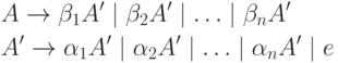
Generalizing, it can be shown that if a nonterminal A appears on the left side r+ s generating rules, r of which use direct left recursion, and s- no, i.e.

A→ Aα 1, A→ Aα 2,..., A→ Aα r

A→ β 1, A→ β 2,..., A→ β s

then these rules can be replaced by the following:

An informal proof is that before and after the transformation A generates a regular expression ( β 1 | β 2 |... | β s) ( α 1 | α 2 |... | α r)*

It should be noted that by eliminating the left recursion (or the left recursive loop), we still do not get an LL(1) grammar, because for some non-terminals, on the left side of the rules of the resulting grammars, there are alternative right parts that begin with the same characters. Therefore, after eliminating the left recursion, one should continue the transformation of the grammar to the LL(1) form.

17. Converting grammars to LL(1) form. Factorization.

Factorization

In many situations, grammars that do not have the LL(1) feature can be converted to LL(1) grammars using the factorization process. Let's consider an example of such a situation.

P→ begin D; WITH end

D→ d, D

D→ d

WITH→ s; WITH

WITH→ s

In the factorization process, we replace several rules for one non-terminal on the left side, the right side of which begins with the same symbol (string of symbols) with one rule, where on the right side the common beginning is followed by an additionally introduced non-terminal. The grammar is also supplemented with rules for an additional non-terminal, according to which various “remnants” of the original right-hand side of the rule are derived from it. For the grammar above, this would give the following LL(1) grammar:

P→ begin D; WITH end

D→ d X X)

X→ , D(according to the 1st rule for D original grammar for d follows, D)

X→ ε (according to the 2nd rule for D original grammar for d nothing (empty string)

WITH→ s Y(we introduce an additional non-terminal Y)

Y→ ; WITH(according to the 1st rule for C original grammar for s follows; C)

Y→ ε (according to the 2nd rule for C original grammar for s nothing (empty string)

Similarly, generating rules

S→ aSb

S→ aSc

S→ ε

can be converted by factorization into rules

S→ aSX

S→ ε

X→ b

X→ c

and the resulting grammar will be LL(1). The factorization process, however, cannot be automated by extending it to the general case. The following example shows what can happen. Consider the rules

1. P→ Qx

2. P→ Ry

3. Q→ sQm

4. Q→ q

5. R→ sRn

6. R→ r

Both sets of guide characters for two options P contain s, and trying to "endure s out of brackets", we replace Q and R in the right parts of rules 1 and 2:

P→ sQmx

P→ sRny

P→ qx

P→ ry

These rules can be replaced by the following:

P→ qx

P→ ry

P→ sp 1

P 1 → Qmx

P 1 → Rny

Rules for P1 similar to the original rules for P and have overlapping sets of guide characters. We can transform these rules in the same way as the rules for P:

P 1 → sQmmx

P 1 → qmx

P 1 → sRny

P 1 → rny

Factoring, we get

In the theory of formal grammars and automata (TFGiA) an important role is played by the so-called context-free grammars(CS-grammars). A CS-grammar is a quadruple consisting of a set N of non-terminal symbols, a set T of terminal symbols, a set P of rules (productions), and an initial symbol S belonging to the set N.

Each production p of P has the form A –> a, where A is a non-terminal character (A of N), and a is a string consisting of terminal and non-terminal characters. The word output process begins with a string containing only the initial character S. After that, at each step, one of the non-terminal characters included in the current string is replaced by the right side of one of the productions in which it is the left side. If after such an operation a string containing only terminal characters is obtained, then the output process ends.

In many theoretical problems it is convenient to consider the so-called normal forms grammarian The process of normalizing a grammar often begins with the elimination of left recursion. In this problem, we will consider only its special case, called direct left recursion. An inference rule A -> R is said to contain immediate left recursion if the first character of the string R is A.

The CS-grammar is given. It is required to find the number of rules containing immediate left recursion.

Input data

The first line of the input file INPUT.TXT contains the number n (1 ≤ n ≤ 1000) of rules in the grammar. Each of the following n lines contains one rule. Non-terminal symbols are denoted by capital letters of the English alphabet, terminal symbols - lowercase. The left part of the production is separated from the right part by the –> symbols. The right part of the production has a length of 1 to 30 characters.