Bring to the equation the equation of a straight line and construct. General equation of a straight line on a plane. Drawing up a general equation of a straight line
As shown above, the equations of the same line can be written in at least three forms: general equations of the line, parametric equations of the line, and canonical equations of the line. Consider the question of the transition from the equations of a straight line of one form to the equations of a straight line in another form.
First, we note that if the equations of a straight line are given in parametric form, then the point through which the straight line and the directing vector of the straight line pass through are given. Therefore, it is not difficult to write the equations of a straight line in canonical form.
Example.
Equations of a straight line are given in parametric form
Solution.
The line passes through the point  and has a direction vector
  . Therefore, the canonical equations of the line have the form
 .
.
The problem of the transition from the canonical equations of the straight line to the parametric equations of the straight line is solved similarly.
The transition from the canonical equations of the straight line to the general equations of the straight line is considered below with an example.
Example.
Given the canonical equations of the line
 .
.
Write down the general equations of the straight line.
Solution.
We write the canonical equations of the straight line as a system of two equations
 .
.
Getting rid of the denominators by multiplying both sides of the first equation by 6, and the second equation by 4, we get the system
 .
.
 .
.
The resulting system of equations is the general equations of the straight line.
Consider the transition from general equations of the straight line to parametric and canonical equations of the straight line. To write the canonical or parametric equations of a straight line, one must know the point through which the straight line passes and the directing vector of the straight line. If we determine the coordinates of two points  and
and  lying on a straight line, then as the direction vector m we can take the vector
  . The coordinates of two points lying on a straight line can be obtained as solutions to a system of equations that define the general equations of the straight line. As a point through which the line passes, you can take any of the points
  and
and  . Let's illustrate the above with an example.
Example.
Given the general equations of the straight line
 .
.
Solution.
Let's find the coordinates of two points lying on a straight line as solutions to this system of equations. Assuming  , we obtain a system of equations
 .
.
Solving this system, we find  . Hence the point
  lies on a straight line. Assuming
  , we obtain a system of equations
 ,
,
solving which we find  . Therefore, the line passes through the point
  . Then, as a direction vector, we can take the vector
 .
.
So the line passes through the point  and has a direction vector
  . Therefore, the parametric equations of the straight line have the form
 .
.
Then the canonical equations of the straight line are written in the form
 .
.
Another way to find the directing vector of a straight line from the general equations of a straight line is based on the fact that in this case the equations of the planes are given, and hence the normals to these planes.
Let the general equations of the straight line have the form

 and
and  are the normals to the first and second planes, respectively. Then the vector
  can be taken as a directing vector straight line. Indeed, the line, being the line of intersection of these planes, is simultaneously perpendicular to the vectors
  and
and  . Therefore, it is collinear to the vector
  and hence this vector can be taken as the directing vector of the straight line. Consider an example.
Example.
Given the general equations of the straight line
 .
.
Write the parametric and canonical equations of the straight line.
Solution.
A straight line is a line of intersection of planes with normals  and
and  . We take a direct vector as a guide vector

Let's find a point on the line. Let's find a point on the line. Let  . Then we get the system
 .
.
Solving the system, we find  .Hence the point
  lies on a straight line. Then the parametric equations of the straight line can be written as
 .
.
The canonical equations of a straight line have the form
 .
.
Finally, one can pass to the canonical equations by excluding one of the variables in one of the equations, and then the other variable. Let's look at this method with an example.
Example.
Given the general equations of the straight line
 .
.
Write down the canonical equations of the line.
Solution.
We eliminate the variable y from the second equation by adding the first one multiplied by four. Get
 .
.
 .
.
Now we eliminate the variable from the second equation  , adding to it the first equation, multiplied by two. Get
 .
.
 .
.
From here we obtain the canonical equation of the straight line
 .
.
 .
.
 .
.
In this article, we will consider the general equation of a straight line in a plane. Let us give examples of constructing the general equation of a straight line if two points of this straight line are known or if one point and the normal vector of this straight line are known. Let us present methods for transforming an equation in general form into canonical and parametric forms.
Let an arbitrary Cartesian rectangular coordinate system be given Oxy. Consider a first degree equation or a linear equation:
| Ax+By+C=0, | (1) |
where A, B, C are some constants, and at least one of the elements A and B different from zero.
We will show that a linear equation in the plane defines a straight line. Let us prove the following theorem.
Theorem 1. In an arbitrary Cartesian rectangular coordinate system on a plane, each straight line can be given by a linear equation. Conversely, each linear equation (1) in an arbitrary Cartesian rectangular coordinate system on the plane defines a straight line.
Proof. It suffices to prove that the line L is determined by a linear equation for any one Cartesian rectangular coordinate system, since then it will be determined by a linear equation and for any choice of Cartesian rectangular coordinate system.
Let a straight line be given on the plane L. We choose a coordinate system so that the axis Ox aligned with the line L, and the axis Oy was perpendicular to it. Then the equation of the line L will take the following form:
| y=0. | (2) |
All points on a line L will satisfy the linear equation (2), and all points outside this straight line will not satisfy the equation (2). The first part of the theorem is proved.
Let a Cartesian rectangular coordinate system be given and let linear equation (1) be given, where at least one of the elements A and B different from zero. Find the locus of points whose coordinates satisfy equation (1). Since at least one of the coefficients A and B is different from zero, then equation (1) has at least one solution M(x 0 ,y 0). (For example, when A≠0, dot M 0 (−C/A, 0) belongs to the given locus of points). Substituting these coordinates into (1) we obtain the identity
| Ax 0 +By 0 +C=0. | (3) |
Let us subtract identity (3) from (1):
| A(x−x 0)+B(y−y 0)=0. | (4) |
Obviously, equation (4) is equivalent to equation (1). Therefore, it suffices to prove that (4) defines some line.
Since we are considering a Cartesian rectangular coordinate system, it follows from equality (4) that the vector with components ( x−x 0 , y−y 0 ) is orthogonal to the vector n with coordinates ( A,B}.
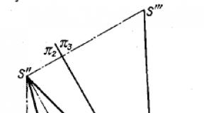
Consider some line L passing through the point M 0 (x 0 , y 0) and perpendicular to the vector n(Fig.1). Let the point M(x,y) belongs to the line L. Then the vector with coordinates x−x 0 , y−y 0 perpendicular n and equation (4) is satisfied (scalar product of vectors n and equals zero). Conversely, if the point M(x,y) does not lie on a line L, then the vector with coordinates x−x 0 , y−y 0 is not orthogonal to vector n and equation (4) is not satisfied. The theorem has been proven.
Proof. Since lines (5) and (6) define the same line, the normal vectors n 1 ={A 1 ,B 1 ) and n 2 ={A 2 ,B 2) are collinear. Since the vectors n 1 ≠0, n 2 ≠ 0, then there is a number λ , what n 2 =n 1 λ . Hence we have: A 2 =A 1 λ , B 2 =B 1 λ . Let's prove that C 2 =C 1 λ . It is obvious that coinciding lines have a common point M 0 (x 0 , y 0). Multiplying equation (5) by λ and subtracting equation (6) from it we get:
Since the first two equalities from expressions (7) are satisfied, then C 1 λ −C 2=0. Those. C 2 =C 1 λ . The remark has been proven.
Note that equation (4) defines the equation of a straight line passing through the point M 0 (x 0 , y 0) and having a normal vector n={A,B). Therefore, if the normal vector of the line and the point belonging to this line are known, then the general equation of the line can be constructed using equation (4).
Example 1. A line passes through a point M=(4,−1) and has a normal vector n=(3, 5). Construct the general equation of a straight line.
Solution. We have: x 0 =4, y 0 =−1, A=3, B=5. To construct the general equation of a straight line, we substitute these values into equation (4):
Answer:
Vector parallel to line L and hence is perpendicular to the normal vector of the line L. Let's construct a normal line vector L, given that the scalar product of vectors n and is equal to zero. We can write, for example, n={1,−3}.
To construct the general equation of a straight line, we use formula (4). Let us substitute into (4) the coordinates of the point M 1 (we can also take the coordinates of the point M 2) and the normal vector n:
Substituting point coordinates M 1 and M 2 in (9) we can make sure that the straight line given by equation (9) passes through these points.
Answer:
Subtract (10) from (1):
We have obtained the canonical equation of a straight line. Vector q={−B, A) is the direction vector of the straight line (12).
See reverse transformation.
Example 3. A straight line in a plane is represented by the following general equation:
Move the second term to the right and divide both sides of the equation by 2 5.
If PDCS is introduced on the plane, then any equation of the first degree with respect to the current coordinates and 
 , (5)
, (5)
where  and
and  simultaneously not equal to zero defines a straight line.
The converse statement is also true: in PDSC, any straight line can be given by a first-degree equation of the form (5).
An equation of the form (5) is called the general equation of a straight line .
Particular cases of equation (5) are given in the following table.
|
The value of the coefficients |
Equation of a straight line |
Line position |
|
|
|
|
The line passes through the origin |
|
|
|
Straight line parallel to the axis |
||
|
|
Straight line parallel to the axis |
||
|
|
The straight line coincides with the axis |
||
|
|
The straight line coincides with the axis |


Equation of a straight line with slope and initial ordinate.
At  glom inclination straight to the axis
  called the smallest angle
  , on which you need to turn the abscissa axis counterclockwise until it coincides with this straight line (Fig. 6). The direction of any straight line is characterized by its slope factor
 , which is defined as the tangent of the slope
  this straight line, i.e.
 .
.
The only exception is a straight line perpendicular to the axis  , which has no slope.
The equation of a straight line with a slope  and crossing the axis
  at a point whose ordinate is
  (initial ordinate)
, is written as
(initial ordinate)
, is written as
 .
.
Equation of a straight line in segments
Equation of a straight line in segments is called an equation of the form
 , (6)
, (6)
where  and
and  respectively, the lengths of the segments cut off by a straight line on the coordinate axes, taken with certain signs.
Equation of a line passing through a given point in a given direction. bundle of straight lines
Equation of a line passing through a given point  and having a slope
  is written in the form
 . (7)
. (7)
A bunch of straight lines
is the collection of lines in a plane passing through one and the same point  beam center. If the coordinates of the beam center are known, then equation (8) can be considered as the beam equation, since any straight line of the beam can be obtained from equation (8) with the corresponding value of the slope
  (the exception is a straight line, which is parallel to the axis
  her equation
  ).
).
If the general equations of two lines belonging to the pencil are known  and (generators of the bundle), then the equation of any straight line from this bundle can be written in the form
Equation of a line passing through two points
Equation of a line passing through two given points
 and
and  , has the form
 .
.
If the points  and
and  define a line parallel to the axis
 or axes
 , then the equation of such a straight line is written, respectively, in the form
 or
or  .
.
Mutual arrangement of two straight lines. Angle between lines. Parallel condition. Perpendicular condition
Mutual arrangement of two straight lines given by general equations
 and ,
and ,
presented in the following table.
Under angle between two lines
one of the adjacent angles formed at their intersection is understood. Acute angle between straight lines  m
m  , is determined by the formula
 .
.
Note that if at least one of these lines is parallel to the axis  , then formula (11) does not make sense, so we will use the general equations of lines
 and .
and .
formula (11) takes the form
 .
.
Parallel condition:
 or
or  .
.
Perpendicular condition:
 or
or  .
.
Normal equation of a straight line. The distance of a point from a line. Bisector equations
Normal equation of a straight line has the form
where  the length of the perpendicular (normal) dropped from the origin to the straight line,
  the angle of inclination of this perpendicular to the axis
  . To give the general equation of a straight line
  normal form, both parts of equality (12) must be multiplied by normalizing factor
 , taken with the opposite sign of the free term
  .
.
Distance  points
  from straight
find by formulas
from straight
find by formulas

 .
(9)
.
(9)
Equation of bisectors of angles between straight lines
 and
:
and
:
 .
.
Task 16. Dana straight  . Write an equation for a line passing through a point
  parallel to this line.
Solution. By the condition of parallel lines  . To solve the problem, we will use the equation of a straight line passing through a given point
  in this direction (8):
 .
.
Find the slope of this straight line. To do this, from the general equation of the straight line (5) we pass to the equation with the slope coefficient (6) (we express  through
  ):
):
Consequently,  .
.
Problem 17. Find a point  , symmetrical to the point
  , relatively straight
  .
.
Solution. To find a point symmetrical to a point  relatively straight
  (Fig.7) it is necessary:

1) lower from point  directly
  perpendicular,
2) find the base of this perpendicular  point
point  ,
,
3) on the continuation of the perpendicular, set aside a segment  .
.
So, let's write the equation of a straight line passing through a point  perpendicular to this line. To do this, we use the equation of a straight line passing through a given point in a given direction (8):
 .
.
Substitute the coordinates of the point  :
:
 . (11)
We find the angular coefficient from the condition of perpendicularity of the lines:
 .
.
Slope of a given line
 ,
,
hence the slope of the perpendicular line
 .
.
Substitute it into equation (11):
Next, let's find a point  the point of intersection of a given line and its perpendicular line. Since the point
  belongs to both lines, then its coordinates satisfy their equations. This means that in order to find the coordinates of the intersection point, it is required to solve a system of equations composed of the equations of these lines:

System Solution  ,
, , i.e.
  .
.
Dot  is the midpoint of the segment
  , then from formulas (4):
 ,
,  ,
,
find the coordinates of a point  :
:
Thus, the desired point  .
.
Problem 18.Compose the equation of a straight line that passes through a point  and cuts off a triangle with an area equal to 150 square units from the coordinate angle. (Fig.8).
Solution. To solve the problem, we will use the equation of a straight line “in segments” (7):
 .
(12)
.
(12)
Since the point  lies on the desired line, then its coordinates must satisfy the equation of this line:
 .
.
The area of a triangle cut off by a straight line from the coordinate angle is calculated by the formula:

(the module is written because  and
and  may be negative).
Thus, we got a system for finding the parameters  and
and  :
:

This system is equivalent to two systems:


Solution of the first system  ,
, and
and  ,
, .
.
Solution of the second system  ,
, and
and  ,
, .
.
We substitute the found values into equation (12):
 ,
,
 ,
, ,
, .
.
We write the general equations of these lines:
 ,
,
 ,
, ,
, .
.
Problem 19. Calculate distance between parallel lines  and
and  .
.
Solution. The distance between parallel lines is equal to the distance of an arbitrary point of one line to the second line.
Let's choose on a straight line  point
point  arbitrarily, therefore, you can set one coordinate, i.e. for example
  , then
  .
.
Now let's find the distance of the point  to straight
  according to formula (10):
 .
.
Thus, the distance between the given parallel lines is equal.
Task 20. Find the equation of the line passing through the point of intersection of the lines  and
and  (not finding the intersection point) and

Solution. 1) Let us write down the equation of a pencil of lines with known generators (9):
Then the desired straight line has the equation
It is required to find such values  and
and  , for which the beam line passes through the point
  , i.e., its coordinates must satisfy equation (13):
Substitute found  into equation (13) and after simplification we obtain the desired straight line:
 .
.

 .
.
Let's use the condition of parallel lines:  . Let's find the slope coefficients of the lines
  and
and  . We have that
  ,
, .
.
Consequently,
Substitute the found value  into equation (13) and simplify, we obtain the equation of the desired line
  .
.
Tasks for independent solution.
Task 21. Write the equation of a straight line passing through the points  and
and  : 1) with a slope; 2) general; 3) "in segments".
Task 22. Write an equation for a line that passes through a point  and forms with the axis
  corner
  , if 1)
  ,
, ;
2)
;
2) ,
, .
.
Task 23. Write the equations for the sides of a rhombus with diagonals of 10 cm and 6 cm, taking the larger diagonal as the axis  , and the smaller
  per axle
  .
.
Task 24. Equilateral triangle  with a side equal to 2 units, is located as shown in Figure 9. draw up the equations of its sides.
Problem 25. Through the dot  draw a straight line that cuts off equal segments on the positive semi-axes of coordinates.
Problem 26. Find the area of a triangle that cuts off a straight line from the coordinate angle:
1)
 ;
2)
;
2) .
.
Problem 27.Write the equation of a straight line passing through a point  and cutting off a triangle from the coordinate angle with an area equal to
  , if
, if
1)
 ,
, sq. units; 2)
  ,
, sq. units
Task 28. Given the vertices of a triangle  . Find the equation of the midline parallel to the side
  , if
, if
We said that a second order algebraic curve is determined by a second degree algebraic equation with respect to X and at. In general, such an equation can be written as
BUT X 2 + B hu+ C at 2+D x+ E y+ F = 0, (6)
where A 2 + B 2 + C 2 ¹ 0 (that is, the numbers A, B, C do not vanish at the same time). Terms A X 2 , V hu, FROM at 2 are called senior terms of the equation, the number
called discriminant this equation. Equation (6) is called general equation curve of the second order.
For the previously considered curves we have:
Ellipse:  Þ A = , B = 0, C = , D = E = 0, F = –1,
circle X 2 + at 2 = a 2 Þ A = C = 1, B = D = E = 0, F = - a 2 , d = 1>0;
Hyperbola:  Þ A = , B = 0, C = - , D = E = 0, F = -1,
d = - .< 0.
Parabola: at 2 = 2pxÞ A \u003d B \u003d 0, C \u003d 1, D \u003d -2 R, E = F = 0, d = 0,
X 2 = 2RUÞ A \u003d 1B \u003d C \u003d D \u003d 0, E \u003d -2 R, F = 0, d = 0.
The curves given by equation (6) are called central curves if d¹0. If d> 0, then the curve elliptical type if d<0, то кривая hyperbolic type. Curves for which d = 0 are curves parabolic type.
It is proved that the second-order line in any Cartesian coordinate system is given by a second-order algebraic equation. Only in one system the equation has a complex form (for example, (6)), and in the other it is simpler, for example, (5). Therefore, it is convenient to consider such a coordinate system in which the curve under study is written by the simplest (for example, canonical) equation. The transition from one coordinate system, in which the curve is given by an equation of the form (6) to another, where its equation has a simpler form, is called coordinate transformation.
Consider the main types of coordinate transformations.
 I. Transfer Transform coordinate axes (with preservation of direction). Let the point M in the initial XOU coordinate system have coordinates ( X, atX¢, at¢). It can be seen from the drawing that the coordinates of the point M in different systems are related by the relations
(7), or (8).
Formulas (7) and (8) are called coordinate transformation formulas.
 II. Rotate Transform coordinate axes by angle a. If in the initial XOU coordinate system the point M has coordinates ( X, at), and in the new XO¢Y coordinate system it has coordinates ( X¢, at¢). Then the relationship between these coordinates is expressed by the formulas
 , (9)
, (9)

or
Using the coordinate transformation, equation (6) can be reduced to one of the following canonical equations.
1) - ellipse,
2) - hyperbole,
3) at 2 = 2px, X 2 = 2RU- parabola
4) a 2 X 2 – b 2 y 2 \u003d 0 - a pair of intersecting lines (Fig. a)
5) y 2 – a 2 \u003d 0 - a pair of parallel lines (Fig. b)
6) x 2 –a 2 \u003d 0 - a pair of parallel lines (Fig. c)
7) y 2 = 0 - coinciding lines (OX axis)
8) x 2 = 0 - coinciding lines (OS axis)
9) a 2 X 2 + b 2 y 2 = 0 - point (0, 0)
10)
 imaginary ellipse
11) y 2 + a 2 = 0– pair of imaginary lines
12) x 2 + a 2 = 0 pair of imaginary lines.
Each of these equations is a second-order line equation. The lines defined by equations 4 - 12 are called degenerate curves of the second order.
 |
|||
 |
|||

Let us consider examples of transformation of the general equation of a curve to a canonical form.
1) 9X 2 + 4at 2 – 54X + 8at+ 49 = 0 Þ (9 X 2 – 54X) + (4at 2 + 8at) + 49 = 0 z
9(X 2 – 6X+ 9) + 4(at 2 + 2at+ 1) – 81 – 4 + 49 = 0 Þ 9( X –3) 2 + 4(at+ 1) = 36, z

![]() .
.
Let's put X¢ = X – 3, at¢ = at+ 1, we obtain the canonical equation of the ellipse ![]() . Equality X¢ = X – 3, at¢ = at+ 1 define the translation transformation of the coordinate system to the point (3, –1). Having built the old and new coordinate systems, it is easy to draw this ellipse.
. Equality X¢ = X – 3, at¢ = at+ 1 define the translation transformation of the coordinate system to the point (3, –1). Having built the old and new coordinate systems, it is easy to draw this ellipse.
2) 3at 2 +4X– 12at+8 = 0. Let's transform:
(3at 2 – 12at)+ 4 X+8 = 0
3(at 2 – 4at+4) – 12 + 4 X +8 = 0
3(y - 2) 2 + 4(X –1) = 0
(at – 2) 2 = – (X – 1) .
Let's put X¢ = X – 1, at¢ = at– 2, we get the parabola equation at¢2 = - X¢. The chosen substitution corresponds to the transfer of the coordinate system to the point О¢(1,2).
Let us establish a rectangular coordinate system on the plane and consider the general equation of the second degree
wherein  .
.
The set of all points in the plane whose coordinates satisfy equation (8.4.1) is called crooked (line) second order.
For any curve of the second order, there is a rectangular coordinate system, called canonical, in which the equation of this curve has one of the following forms:
1)
 (ellipse);
2)
 (imaginary ellipse);
3)
 (a pair of imaginary intersecting lines);
4)
 (hyperbola);
5)
 (a pair of intersecting lines);
6)
 (parabola);
7)
 (pair of parallel lines);
8)
 (a pair of imaginary parallel lines);
9)
 (a pair of coinciding lines).
Equations 1)–9) are called canonical equations of curves of the second order.
The solution of the problem of reducing the equation of a curve of the second order to the canonical form includes finding the canonical equation of the curve and the canonical coordinate system. Reduction to the canonical form allows you to calculate the parameters of the curve and determine its location relative to the original coordinate system. Transition from the original rectangular coordinate system  to canonical
  is carried out by rotating the axes of the original coordinate system around the point O to a certain angle and subsequent parallel transfer of the coordinate system.
Curve invariants of the second order(8.4.1) are called such functions of the coefficients of its equation, the values of which do not change when moving from one rectangular coordinate system to another of the same system.
For a curve of the second order (8.4.1), the sum of the coefficients at squared coordinates
 ,
,
determinant composed of the coefficients of the leading terms

and third order determinant

are invariants.
The value of the invariants s, , can be used to determine the type and compose the canonical equation of a second-order curve (Table 8.1).
Table 8.1
Classification of second-order curves based on invariants
Let's take a closer look at the ellipse, hyperbola, and parabola.
Ellipse(Fig. 8.1) is the locus of points in the plane for which the sum of the distances to two fixed points  this plane, called ellipse tricks, is a constant value (greater than the distance between the foci). This does not exclude the coincidence of the foci of the ellipse. If the foci are the same, then the ellipse is a circle.
The half-sum of distances from a point of an ellipse to its foci is denoted by a, half the distance between the foci - With. If the rectangular coordinate system on the plane is chosen so that the ellipse focuses on the axis Ox symmetrical about the origin, then in this coordinate system the ellipse is given by the equation
 ,
(8.4.2)
,
(8.4.2)
called the canonical equation of the ellipse, where  .
.

Rice. 8.1
With the specified choice of a rectangular coordinate system, the ellipse is symmetrical about the coordinate axes and the origin. The axes of symmetry of an ellipse call it axes, and the center of symmetry is the center of the ellipse. At the same time, the numbers 2 are often called the axes of the ellipse. a and 2 b, and the numbers a and b – big and semi-minor axis respectively.
The points of intersection of an ellipse with its axes are called the vertices of the ellipse. The vertices of the ellipse have coordinates ( a, 0), (–a, 0), (0, b), (0, –b).
Ellipse eccentricity called a number
 . (8.4.3)
Because 0 c < a, ellipse eccentricity 0 < 1, причем у окружности = 0. Перепишем равенство (8.4.3) в виде
 .
.
This shows that the eccentricity characterizes the shape of the ellipse: the closer to zero, the more the ellipse looks like a circle; as increases, the ellipse becomes more elongated.
Let  is an arbitrary point of the ellipse,
  and
and  - distance from point M before tricks F 1 and F 2 respectively. Numbers r 1 and r 2 are called point focal radii
M
ellipse and are calculated by the formulas
- distance from point M before tricks F 1 and F 2 respectively. Numbers r 1 and r 2 are called point focal radii
M
ellipse and are calculated by the formulas
Headmistresses other than circle ellipse with the canonical equation (8.4.2) two lines are called
 .
.
The directrixes of the ellipse are located outside the ellipse (Fig. 8.1).
Focal radius ratio  pointsMellipse to distance

of this ellipse (focus and directrix are considered to correspond if they are located on the same side of the center of the ellipse).
of this ellipse (focus and directrix are considered to correspond if they are located on the same side of the center of the ellipse).
Hyperbole(Fig. 8.2) is the locus of points of the plane for which the modulus of the difference in distances to two fixed points  and
and  this plane, called foci of hyperbole, is a constant value (not equal to zero and less than the distance between the foci).
Let the distance between foci be 2 With, and the specified modulus of the distance difference is 2 a. We choose a rectangular coordinate system in the same way as for an ellipse. In this coordinate system, the hyperbola is given by the equation
 ,
(8.4.4)
,
(8.4.4)
called the canonical equation of the hyperbola, where  .
.

Rice. 8.2
With this choice of a rectangular coordinate system, the coordinate axes are the axes of symmetry of the hyperbola, and the origin of coordinates is its center of symmetry. The axes of symmetry of a hyperbola are called axes, and the center of symmetry is the center of the hyperbola. Rectangle with 2 sides a and 2 b, located as shown in Fig. 8.2, called the main rectangle of a hyperbola. Numbers 2 a and 2 b are the axes of the hyperbola, and the numbers a and b- her axle shafts. Straight lines, which are a continuation of the diagonals of the main rectangle, form hyperbola asymptotes
 .
.
Points of intersection of the hyperbola with the axis Ox called vertices of the hyperbola. The vertices of the hyperbola have coordinates ( a, 0), (–a, 0).
The eccentricity of a hyperbola called a number
 . (8.4.5)
Because the With > a, the eccentricity of the hyperbola > 1. Let us rewrite equality (8.4.5) as
 .
.
This shows that the eccentricity characterizes the shape of the main rectangle and, consequently, the shape of the hyperbola itself: the smaller , the more the main rectangle is extended, and after it the hyperbola itself along the axis Ox.
Let  is an arbitrary point of the hyperbola,
  and
and  - distance from point M before tricks F 1 and F 2 respectively. Numbers r 1 and r 2 are called point focal radii
M
hyperbole and are calculated by the formulas
- distance from point M before tricks F 1 and F 2 respectively. Numbers r 1 and r 2 are called point focal radii
M
hyperbole and are calculated by the formulas

Headmistresses hyperbole with the canonical equation (8.4.4) two lines are called
 .
.
The directrixes of the hyperbola intersect the main rectangle and pass between the center and the corresponding vertex of the hyperbola (Fig. 8.2).
O  focal radius ratio
  pointsM
hyperbolas to distance
pointsM
hyperbolas to distance  from this point to the corresponding focus
  directrix is equal to eccentricity
this hyperbola (focus and directrix are considered to be corresponding if they are located on the same side of the center of the hyperbola).
directrix is equal to eccentricity
this hyperbola (focus and directrix are considered to be corresponding if they are located on the same side of the center of the hyperbola).
parabola(Fig. 8.3) is the locus of points in the plane for which the distance to some fixed point F (focus of the parabola) of this plane is equal to the distance to some fixed line ( parabola directrixes), also located in the considered plane.
Let's choose the beginning O rectangular coordinate system in the middle of the segment [ FD], which is a perpendicular dropped from the focus F to the directrix (it is assumed that the focus does not belong to the directrix), and the axes Ox and Oy direct as shown in Fig. 8.3. Let the length of the segment [ FD] is equal to p. Then in the chosen coordinate system  and canonical parabola equation has the form
 . (8.4.6)
Value p called parabola parameter.
A parabola has an axis of symmetry called parabola axis. The point of intersection of a parabola with its axis is called top of the parabola. If the parabola is given by its canonical equation (8.4.6), then the axis of the parabola is the axis Ox. Obviously, the vertex of the parabola is the origin.
Example 1 Dot BUT= (2, –1) belongs to the ellipse, the point F= (1, 0) is its focus, corresponding to F the directrix is given by the equation  . Write an equation for this ellipse.
Solution. We will assume the coordinate system is rectangular. Then the distance  from the point BUT to headmistress
  in accordance with relation (8.1.8), in which

 , equals
 .
.
Distance  from the point BUT to focus F equals
 ,
,
which allows you to determine the eccentricity of the ellipse
 .
.
Let M
= (x,
y) is an arbitrary point of the ellipse. Then the distance  from the point M to headmistress
  according to the formula (8.1.8) is equal to

and the distance  from the point M to focus F equals
 .
.
Since for any point of the ellipse the relation  is a constant value equal to the eccentricity of the ellipse, hence we have
 ,
,
Example 2 The curve is given by the equation
in a rectangular coordinate system. Find the canonical coordinate system and the canonical equation of this curve. Define the curve type.
Solution. quadratic form  has a matrix
 .
.
Its characteristic polynomial

has roots 1 = 4 and 2 = 9. Therefore, in an orthonormal basis of matrix eigenvectors BUT the considered quadratic form has the canonical form
 .
.
Let us proceed to the construction of the matrix of the orthogonal transformation of variables, which reduces the considered quadratic form to the indicated canonical form. To do this, we will construct fundamental systems of solutions of homogeneous systems of equations  and orthonormalize them.
At  this system looks like

Its general solution is  . There is one free variable here. Therefore, the fundamental system of solutions consists of one vector, for example, the vector
  . Normalizing it, we get the vector
 .
.
At  we will also construct a vector
 .
.
Vectors  and
and  are already orthogonal, since they refer to different eigenvalues of the symmetric matrix BUT. They constitute the canonical orthonormal basis of the given quadratic form. From the columns of their coordinates, the desired orthogonal matrix (rotation matrix) is built
 .
.
Check the correctness of finding the matrix R according to the formula  , where
  is a matrix of quadratic form in the basis
  :
:

Matrix R found correctly.
Let's perform the transformation of variables

and write the equation of this curve in the new rectangular coordinate system with the old center and direction vectors  :
:


where  .
.
We got the canonical equation of the ellipse
 .
.
Due to the fact that the resulting transformation of rectangular coordinates is determined by the formulas
 ,
,
 ,
,
canonical coordinate system  has a beginning
  and direction vectors
  .
.
Example 3 Using invariant theory, determine the type and write the canonical equation of the curve
Solution. Because the

 ,
,
in accordance with the table. 8.1 we conclude that this is a hyperbole.
Since s = 0, the characteristic polynomial of the matrix of the quadratic form 
its roots  and
and  allow us to write the canonical equation of the curve
where FROM is found from the condition
 ,
,
 .
.
The desired canonical equation of the curve
 .
.
In the problems of this section, the coordinatesx, yassumed to be rectangular.
8.4.1.
For ellipses  and
and  find:
find:
a) half shafts;
b) tricks;
c) eccentricity;
d) directrix equations.
8.4.2.
Write the equations of an ellipse, knowing its focus  corresponding to the directrix x= 8 and eccentricity
  . Find the second focus and second directrix of the ellipse.
8.4.3. Write an equation for an ellipse whose foci are (1, 0) and (0, 1) and whose major axis is two.
8.4.4.
Dana hyperbole  . Find:
a) axles a and b;
b) tricks;
c) eccentricity;
d) asymptote equations;
e) directrix equations.
8.4.5.
Dana hyperbole  . Find:
a) axles a and b;
b) tricks;
c) eccentricity;
d) asymptote equations;
e) directrix equations.
8.4.6.
Dot  belongs to a hyperbola whose focus is
  , and the corresponding directrix is given by the equation
  . Write an equation for this hyperbola.
8.4.7.
Write an equation for a parabola given its focus  and headmistress
  .
.
8.4.8.
Given the vertex of a parabola  and the directrix equation
  . Write an equation for this parabola.
8.4.9. Write an equation for a parabola whose focus is at a point

and the directrix is given by the equation  .
.
8.4.10.
Write an equation for a second-order curve, knowing its eccentricity  , focus
  and the corresponding director
  .
.
8.4.11. Determine the type of the second-order curve, write its canonical equation and find the canonical coordinate system:
G)  ;
;
8.4.12.
is an ellipse. Find the lengths of the semi-axes and the eccentricity of this ellipse, the coordinates of the center and foci, write the equations of the axes and directrixes.
8.4.13. Prove that the second-order curve given by the equation
is a hyperbole. Find the lengths of the semi-axes and the eccentricity of this hyperbola, the coordinates of the center and foci, write the equations for the axes, directrixes and asymptotes.
8.4.14. Prove that the second-order curve given by the equation
 ,
,
is a parabola. Find the parameter of this parabola, the coordinates of the vertices and focus, write the equations for the axis and directrix.
8.4.15. Bring each of the following equations to canonical form. Draw in the drawing the corresponding second-order curve with respect to the original rectangular coordinate system:
8.4.16. Using invariant theory, determine the type and write the canonical equation of the curve.