Graph of function y 2x squared figure. Function graph. Video tutorials with parabola
The function y \u003d x ^ 2 is called a quadratic function. The graph of a quadratic function is a parabola. The general view of the parabola is shown in the figure below.
Quadratic function
Fig 1. General view of the parabola
As you can see from the graph, it is symmetrical about the Oy axis. The Oy axis is called the axis of symmetry of the parabola. This means that if you draw a straight line parallel to the Ox axis above this axis. Then it will cross the parabola at two points. The distance from these points to the Oy axis will be the same.
The axis of symmetry divides the parabola graph into two parts. These parts are called the branches of the parabola. And the point of the parabola that lies on the axis of symmetry is called the vertex of the parabola. That is, the axis of symmetry passes through the apex of the parabola. The coordinates of this point (0; 0).
Basic properties of a quadratic function
1. For x \u003d 0, y \u003d 0, and y\u003e 0 for x0
2. The quadratic function reaches its minimum value at its vertex. Ymin at x \u003d 0; It should also be noted that the function does not have a maximum value.
3. The function decreases on the interval (-∞; 0] and increases on the interval, the function decreases,
and for x ∈ [0; + ∞) increases.
the vertex is at the point with coordinates (0; 3). Find the value of the function
y \u003d 5x + 4 if:
x \u003d -1
y \u003d - 1 y \u003d 19
x \u003d -2
y \u003d -6
y \u003d 29
x \u003d 3
x \u003d 5 Please indicate
function scope:
y \u003d 16 - 5x
10
y
x
x - any
number
x ≠ 0
1
y
x 7
4x 1
y
5
x ≠ 7 Plot function graphs:
1) .Y \u003d 2X + 3
2) .Y \u003d -2X-1;
3).
10.
Mathematicalstudy
Topic: Function y \u003d x2
11.
Buildschedule
function
y \u003d x2
12.
Parabola construction algorithm.1.Fill in the table of X and Y values.
2. Mark the points in the coordinate plane,
whose coordinates are indicated in the table.
3. Connect these points with a smooth line.
13.
Incrediblebut the fact!
Pass Parabola
14.
Did you know?The trajectory of a stone thrown under
angle to the horizon, will fly along
parabola.
15. Properties of the function y \u003d x2
*Function properties
y \u003d
2
x
16.
*Domainfunction D (f):
x - any number.
* Range of values
function E (f):
all values \u200b\u200bof y ≥ 0.
17.
*If ax \u003d 0, then y \u003d 0.
Function graph
goes through
origin.
18.
III
*If a
x ≠ 0,
then y\u003e 0.
All points of the graph
functions other than point
(0; 0), located
above the x-axis.
19.
* Oppositevalues \u200b\u200bx
corresponds to one
and the same value of y.
Function graph
symmetrical
about the axis
ordinate.
20.
Geometricparabola properties
* Possesses symmetry
* The axis cuts the parabola into
two parts: branches
parabolas
* Point (0; 0) - top
parabolas
* The parabola touches the axis
abscissa
Axis
symmetry
21.
Find y if:“Knowledge is a tool
not a goal "
L. N. Tolstoy
x \u003d 1.4
- 1,4
y \u003d 1.96
x \u003d 2.6
-2,6
y \u003d 6.76
x \u003d 3.1
- 3,1
y \u003d 9.61
Find x if:
y \u003d 6
y \u003d 4
x ≈ 2.5 x ≈ -2.5
x \u003d 2 x \u003d -2
22.
build in onecoordinate system
graphs of two functions
1. Case:
y \u003d x2
Y \u003d x + 1
2.case:
Y \u003d x2
y \u003d -1
23.
Findseveral meanings
x for which
function values:
less than 4
over 4
24.
Does the graph of the function y \u003d x2 point belong:P (-18; 324)
R (-99; -9081)
belongs
not belong
S (17; 279)
not belong
Without performing any calculations, determine which of
points do not belong to the graph of the function y \u003d x2:
(-1; 1)
*
(-2; 4)
(0; 8)
(3; -9)
(1,8; 3,24)
For what values \u200b\u200bof a the point P (a; 64) belongs to the graph of the function y \u003d x2.
a \u003d 8; a \u003d - 8
(16; 0)
25.
Algorithm for solving the equationgraphically
1. Build in one system
coordinates of the graphics of functions standing
on the left and right sides of the equation.
2. Find abscissas of intersection points
charts. These will be the roots
equations.
3. If there are no intersection points, then
the equation has no roots
Previously, we studied other functions, for example linear, recall its standard form:
hence the obvious fundamental difference - in the linear function x stands in the first degree, and in that new function, which we are starting to study, x stands in the second degree.
Recall that the graph of a linear function is a straight line, and the graph of a function, as we will see, is a curve called a parabola.
Let's start by finding out where the formula came from. The explanation is this: if we are given a square with a side and, then we can calculate its area as follows:
If we change the length of the side of the square, then its area will also change.
So, here is one of the reasons why we are studying the function
Recall that the variable x is an independent variable, or an argument, in physical interpretation it can be, for example, time. Distance is, on the contrary, a dependent variable, it depends on time. The dependent variable or function is a variable at.
This is the law of correspondence, according to which each value x is assigned a single value at.
Any correspondence law must satisfy the requirement of uniqueness from argument to function. In the physical interpretation, this looks quite clear on the example of the dependence of distance on time: at each moment of time we are at a certain distance from the starting point, and it is impossible at the same time at time t to be both 10 and 20 kilometers from the beginning of the path.
At the same time, each function value can be reached with several argument values.
So, we need to build a graph of the function, for this we create a table. Then, according to the schedule, examine the function and its properties. But even before plotting the graph by the type of function, we can say something about its properties: it is obvious that at cannot take negative values, since
So, let's make a table:

Figure: one
It is easy to note the following properties from the graph:
Axis at is the axis of symmetry of the graph;
The vertex of the parabola is the point (0; 0);
We see that the function only takes non-negative values;
In the interval where ![]() the function decreases, and on the interval where the function increases;
the function decreases, and on the interval where the function increases;
The function acquires the smallest value at the vertex, ![]() ;
;
There is no largest function value;
Example 1
Condition:
![]()
Decision:
Insofar as x by condition it changes at a specific interval, we can say about the function that it increases and changes over the interval. The function has a minimum value and a maximum value in this interval.

Figure: 2. The graph of the function y \u003d x 2, x ∈
Example 2
Condition: Find the largest and smallest function value:
![]()
Decision:
x changes in the interval, which means at decreases in the so far interval and increases in the so far interval.
So the limits of change x , and the limits of change at , and, therefore, on this interval, there exists both the minimum value of the function and the maximum

Figure: 3. Graph of the function y \u003d x 2, x ∈ [-3; 2]
Let us illustrate the fact that the same function value can be achieved with several values \u200b\u200bof the argument.
The construction of graphs of functions containing modules usually causes considerable difficulties for schoolchildren. However, things are not so bad. It is enough to memorize several algorithms for solving such problems, and you can easily build a graph of even the most seemingly complex function. Let's figure out what these algorithms are.
1. Plotting the function y \u003d | f (x) |
Note that the set of values \u200b\u200bof the functions y \u003d | f (x) | : y ≥ 0. Thus, the graphs of such functions are always located completely in the upper half-plane.
Plotting the function y \u003d | f (x) | consists of the following simple four steps.
1) Construct accurately and carefully the graph of the function y \u003d f (x).
2) Leave unchanged all the points of the graph that are above the 0x axis or on it.
3) The part of the graph, which lies below the 0x axis, display symmetrically about the 0x axis.
Example 1. Display the graph of the function y \u003d | x 2 - 4x + 3 |
1) We build a graph of the function y \u003d x 2 - 4x + 3. Obviously, the graph of this function is a parabola. Find the coordinates of all points of intersection of the parabola with the coordinate axes and the coordinates of the vertex of the parabola.
x 2 - 4x + 3 \u003d 0.
x 1 \u003d 3, x 2 \u003d 1.
Therefore, the parabola crosses the 0x axis at points (3, 0) and (1, 0).
y \u003d 0 2 - 4 0 + 3 \u003d 3.
Therefore, the parabola intersects the 0y-axis at the point (0, 3).
Parabola vertex coordinates:
x in \u003d - (- 4/2) \u003d 2, y in \u003d 2 2 - 4 2 + 3 \u003d -1.
Therefore, point (2, -1) is the vertex of this parabola.
Draw a parabola using the received data (fig. 1)
2) The part of the graph that lies below the 0x axis is displayed symmetrically about the 0x axis.
3) We get the graph of the original function ( fig. 2, depicted by a dotted line).

2. Plotting the function y \u003d f (| x |)
Note that functions of the form y \u003d f (| x |) are even:
y (-x) \u003d f (| -x |) \u003d f (| x |) \u003d y (x). This means that the graphs of such functions are symmetric about the 0y axis.
Graphing the function y \u003d f (| x |) consists of the following simple chain of actions.
1) Plot the function y \u003d f (x).
2) Leave that part of the graph for which x ≥ 0, that is, the part of the graph located in the right half-plane.
3) Display the part of the graph indicated in point (2) symmetrically to the 0y axis.
4) Select the union of the curves obtained in paragraphs (2) and (3) as the final graph.
Example 2. Display the graph of the function y \u003d x 2 - 4 · | x | + 3
Since x 2 \u003d | x | 2, then the original function can be rewritten as follows: y \u003d | x | 2 - 4 · | x | + 3. And now we can apply the algorithm proposed above.
1) We construct accurately and carefully the graph of the function y \u003d x 2 - 4 x + 3 (see also fig. one).
2) We leave that part of the graph for which x ≥ 0, that is, the part of the graph located in the right half-plane.
3) Display the right side of the graph symmetrically to the 0y axis.
(fig. 3).

Example 3. Display the graph of the function y \u003d log 2 | x |
We apply the scheme given above.
1) Plot the function y \u003d log 2 x (fig. 4).
3. Plotting the function y \u003d | f (| x |) |
Note that functions of the form y \u003d | f (| x |) | are also even. Indeed, y (-x) \u003d y \u003d | f (| -x |) | \u003d y \u003d | f (| x |) | \u003d y (x), and therefore, their graphs are symmetric about the 0y axis. The set of values \u200b\u200bof such functions: y ≥ 0. Hence, the graphs of such functions are located completely in the upper half-plane.
To plot the function y \u003d | f (| x |) |, you need:
1) Construct accurately the graph of the function y \u003d f (| x |).
2) Leave the part of the graph above or on the 0x axis unchanged.
3) The part of the graph, located below the 0x axis, display symmetrically about the 0x axis.
4) Select the union of the curves obtained in paragraphs (2) and (3) as the final graph.
Example 4. Display the graph of the function y \u003d | -x 2 + 2 | x | - 1 |.
1) Note that x 2 \u003d | x | 2. Hence, instead of the original function y \u003d -x 2 + 2 | x | - one
you can use the function y \u003d - | x | 2 + 2 | x | - 1, since their graphs are the same.
We build a graph y \u003d - | x | 2 + 2 | x | - 1. For this we use algorithm 2.
a) Plot the function y \u003d -x 2 + 2x - 1 (fig. 6).

b) Leave the part of the graph that is located in the right half-plane.
c) Display the resulting part of the graph symmetrically to the 0y axis.
d) The resulting graph is shown in the figure with a dotted line (fig. 7).

2) There are no points above the 0x axis, we leave the points on the 0x axis unchanged.
3) The part of the graph located below the 0x axis is displayed symmetrically with respect to 0x.
4) The resulting graph is shown in the figure with a dotted line (fig. 8).

Example 5. Plot the function y \u003d | (2 | x | - 4) / (| x | + 3) |
1) First, you need to plot the function y \u003d (2 | x | - 4) / (| x | + 3). For this, we return to Algorithm 2.
a) Carefully plot the function y \u003d (2x - 4) / (x + 3) (fig. 9).

Note that this function is linear-fractional and its graph is a hyperbola. To plot the curve, you first need to find the asymptotes of the graph. Horizontal - y \u003d 2/1 (the ratio of the coefficients at x in the numerator and denominator of the fraction), vertical - x \u003d -3.
2) Leave the part of the graph above or on the 0x axis unchanged.
3) The part of the graph located below the 0x axis will be displayed symmetrically with respect to 0x.
4) The final graph is shown in the figure (fig. 11).
site, with full or partial copying of the material, a link to the source is required.
Previously, we studied other functions, for example linear, recall its standard form:
hence the obvious fundamental difference - in the linear function x stands in the first degree, and in that new function, which we are starting to study, x stands in the second degree.
Recall that the graph of a linear function is a straight line, and the graph of a function, as we will see, is a curve called a parabola.
Let's start by finding out where the formula came from. The explanation is this: if we are given a square with a side and, then we can calculate its area as follows:
If we change the length of the side of the square, then its area will also change.
So, here is one of the reasons why we are studying the function
Recall that the variable x is an independent variable, or an argument, in physical interpretation it can be, for example, time. Distance is, on the contrary, a dependent variable, it depends on time. The dependent variable or function is a variable at.
This is the law of correspondence, according to which each value x is assigned a single value at.
Any correspondence law must satisfy the requirement of uniqueness from argument to function. In the physical interpretation, this looks quite clear on the example of the dependence of distance on time: at each moment of time we are at a certain distance from the starting point, and it is impossible at the same time at time t to be both 10 and 20 kilometers from the beginning of the path.
At the same time, each function value can be reached with several argument values.
So, we need to build a graph of the function, for this we create a table. Then, according to the schedule, examine the function and its properties. But even before plotting the graph by the type of function, we can say something about its properties: it is obvious that at cannot take negative values, since
So, let's make a table:
Figure: one
It is easy to note the following properties from the graph:
Axis at is the axis of symmetry of the graph;
The vertex of the parabola is the point (0; 0);
We see that the function only takes non-negative values;
In the interval where ![]() the function decreases, and on the interval where the function increases;
the function decreases, and on the interval where the function increases;
The function acquires the smallest value at the vertex, ![]() ;
;
There is no largest function value;
Example 1
Condition:
![]()
Decision:
Insofar as x by condition it changes at a specific interval, we can say about the function that it increases and changes over the interval. The function has a minimum value and a maximum value in this interval.
Figure: 2. The graph of the function y \u003d x 2, x ∈
Example 2
Condition: Find the largest and smallest function value:
![]()
Decision:
x changes in the interval, which means at decreases in the so far interval and increases in the so far interval.
So the limits of change x , and the limits of change at , and, therefore, on this interval, there exists both the minimum value of the function and the maximum
Figure: 3. Graph of the function y \u003d x 2, x ∈ [-3; 2]
Let us illustrate the fact that the same function value can be achieved with several values \u200b\u200bof the argument.